If you ever need to export huge images from QGIS, as I recently had to to for a mural-sized map, you are up for a surprise. Anything larger than 32767 pixels in one dimension will give you trouble. Trying to solve this taught me lots of things, leading me through the path of image compositing using ImageMagick, as well as command line usage of Inkscape, both of which turned out to be very interesting, powerful and probably useful to someone out there.

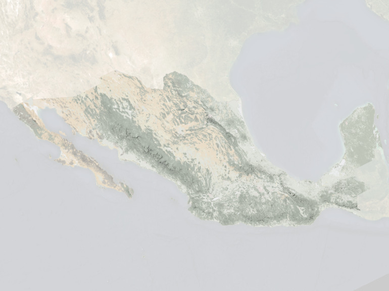
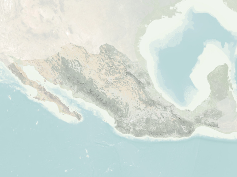
Here I'm going to show how I put together this Mexico background layer for a very large map:

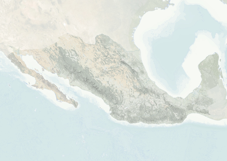
This layer is a composite of a Sentinel satellite image with color correction, a land use layer and a Mexican states layer from INEGI, a shaded relief based on a SRTM model and a bathymetry layer from GEBCO data.

The article covers the following applications: QGIS (a GIS application for mapping), Inkscape (vector editing), SVGO (for reducing the file size of vector images) and ImageMagick (command line image processing).

can this stuff be done with ArcGIS, Illustrator and/or Photoshop? I have no idea, since I don’t own/subscribe to/pirate these things. My workflow for this project and the tutorial below consists solely of free and open source tools

Problem: your bitmap is too big for QGIS

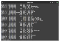
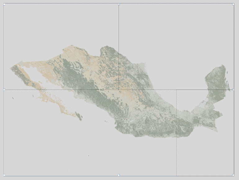
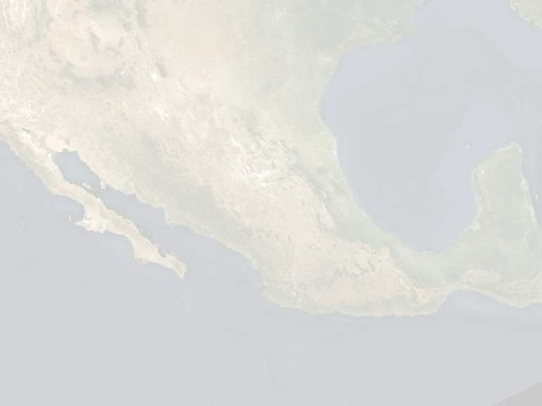
The map I was making had to be printed at a size of 4.4 x 3.3 meters (about 14 x 11 feet) in 300 dpi resolution. I needed then to export it in PNG format from QGIS with a size of 52438 x 39213 pixels, which adds up to about 2G pixels (two billion pixels). I usually export each layer of a map separately and then compose them using KritaKrita, unlike GIMP, has file layers which update automatically when I overwrite a layer’s file with a new version., which I find much faster and flexible than doing it in QGIS. So in this case I started by exporting the land use layer. It came out like this:

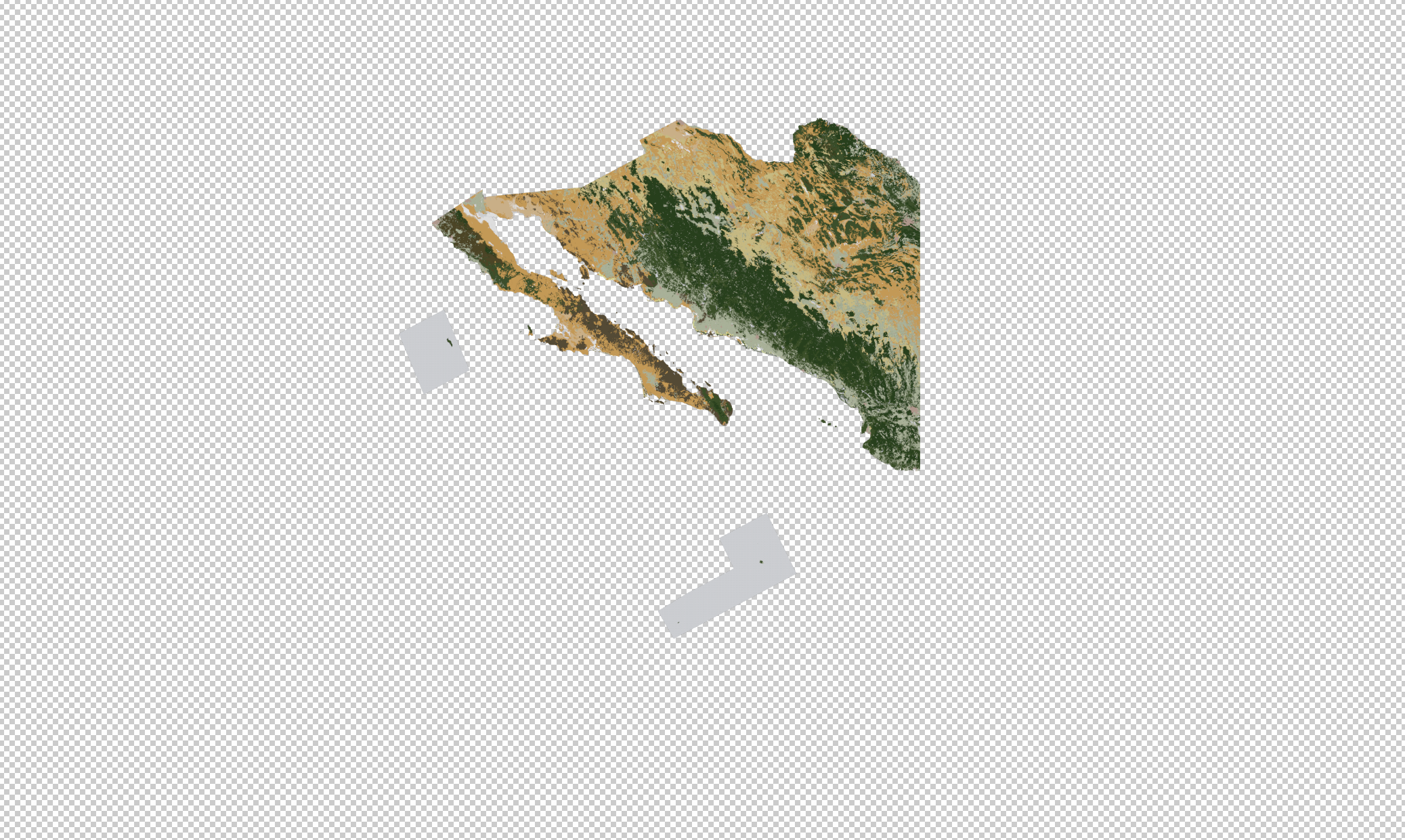
It took forever to export and then, the image was cut off on the x axis at exactly 32767 pixels (it was probably also cut off horizontally). I was not running out of memory, so it was something else. This number did sound familiar, and it turns out 32767 is the largest number that can be written as 16-bit (binary) signed integer value in a computer’s memory. So it must be difficult to overcome (something should be recoded from 16 to 32 bits, perhaps). Turns out an issue about this in the QGIS reposities has remained open since 2014 and it doesn’t look like it’s going anywhere. Who wants to export images that large? Well, me. My map needed to be printed a bit larger than 4 meters across and people would be looking at it from up close, so at 300 dpi (I’d actually rather use 600 dpi) it is a big number. So I needed to find a workaround.

Solution: export as vectors and convert to a bitmap

⊕
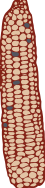
An icon representing apachito corn
(credit: Kitzia Sámano)Instead of exporting as a PNG image, we could export our map as a PDF or SVG vector. But my map is really complex, with one of the corn (maize) layers having more than 22,000 symbols, such as the one here representing apachito corn, one of the many races in Mexico, with 230 individual corn kernels in each icon. This adds up to a very large image. QGIS crashes in the middle of trying to export the map as vectors.

So the solution is to export each vector layer separately. It mostly works (see below), and we now have one SVG file for each layer. We can then open them in Inkscape, hit ctrl+shift+e and convert to PNG with 300 dpi resolution so we get our large bitmap layer. Well… it turns out Inkscape hits exactly the same bitmap export size limit as QGIS, as can be seen in this issue from 2019.

Solution: convert to TWO bitmaps

To try to work around the image size export limit in Inkscape, we could try to export it separately in two smaller halves and then figure out a way of gluing them together again. If you fiddle with the image extent figures in the Export PNG image panel, you can export in two halves which turn out ok as they are both smaller than the 32767 limit:

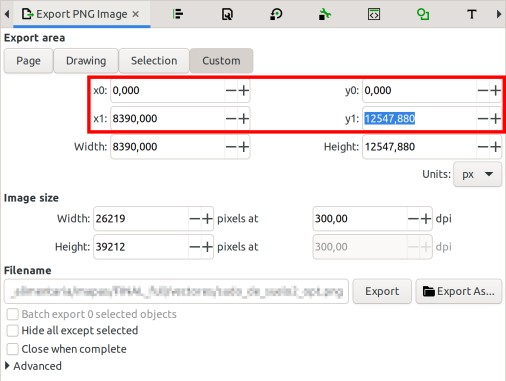
But then, was I going to start typing numbers one by one for all of my layers? No way! That’s what we have the command line for!

The Inkscape command line

⊕
Try using the command line!

If you are doing any kind of serious massive/complex image processing, converting, animation or composing, it is time you get off the mouse and explore your terminal, as it can make your life easier and liberate you from really boring tasks.

When we say “command line” or “terminal” or “cli” or “shell” we mean using an application where you give commands to your computer by typing as opposed to clicking. In Windows, OS X and Linux this application is called the terminal, just search for it and open it. Really, spend a bit of time realizing you can actually use the terminal and nothing bad will happen.Turns out you can do things like converting an SVG vector to a PNG bitmap using Inkscape from the command line. the format is:

inkscape --export-area=x0:y0:x1:y1 --export-dpi=DPI --export-filename=filename.png your_vector.svg

Let’s try with one of the shore and sea layers created in QGIS with GEBCO bathymetry data and exported as SVG (with some built in transparency), a 46 MB file. I open my terminal and run the first command to export the left side of my vector,

inkscape --export-area=0:0:8390:12548 --export-dpi=300 --export-filename=out_left.png mar_color.svg

which results in this PNG image (reduced in size and converted to jpg for the purposes of this website):

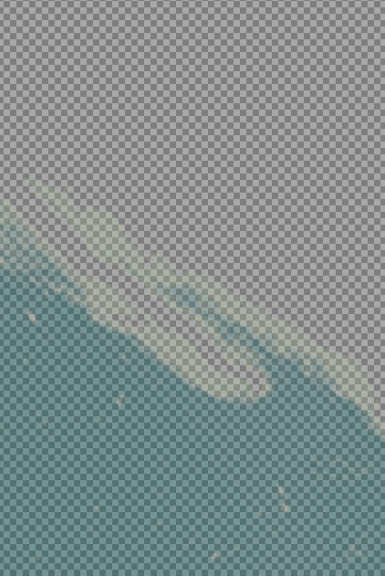
This operation uses about 10 GB of RAM and takes about 9 minutes on my computer. Let’s go with the right side:

inkscape --export-area=8391:0:16781:12548 --export-dpi=300 --export-filename=out_right.png mar_color.svg

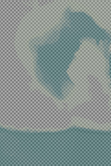
Now I have one exported 300 dpi image for each half of my vector. I got the numbers you see above by trial and error. But it actually works like this: the numbers are in pixels, which in Inkscape mean 1/96th of an inch. The formula is:

inkscape pixels image width = final image width in pixels * 96 / dpi

So when I do that for my desired image size of 52438 for 300 dpi, the image width in Inkscape pixels is 16780.8.

How come I don’t get the same error for the image height, which is larger than 32767 pixels? I don’t know and I don’t care!

Staying on the command line: stitching images together

I first tried to stitch these two halves of my layer using Gimp and Krita, but it was excruciatingly slow and painful. And since we are already here, we might as well stay on the command line and try to automate everything as much as possible for all my layers. Enter ImageMagick.⊕
ImageMagick is a multiplatform (Linux, Windows, OS X and Android) tool for displaying, modifying, converting and combining images from the command line, also known as the terminal. It is pretty old, having been created in 1987 so there are lots of guides from the community about doing most things, but not too many for what I explain in this tutorial (image composing). It is free and open source, so various other applications use it for basic image processing tasks. A fork from the original project, called GraphicsMagick was made in 2002, I haven’t used it but they claim it is faster. The latest version of ImageMagick is 7.x, but here I used version 6.9.11, which has some significant differences. Check the legacy.ImageMagick.org pages for the documentation of version 6.x.

This wonderful command line tool is mostly known for its commands convert and mogrify, often seen in forums around the internet as the solution to converting or resizing images to and from many formats and sizes either individually or in bulk. One of the uses of a command line tool as opposed to a GUI-based one that you interact to using the mouse, is that you can use it as part of a simple script or program to accomplish repetitive tasks. In the simplest automation case you can just copy and paste a command you are using as part of an image processing workflow.

Appending images with ImageMagick

The first task for ImageMagick is to join together the two PNG halves that we produced from our SVG. This is called “appending” in ImageMagick. The format is this:

convert [file 1] [file 2] [file 3] ... [+append (horizontally) | -append (vertically)] [output file]

In our case we want to stick images next to each other horizontally, so we list the files left to right and use +append. So it goes like this:

convert out_left.png out_right.png +append mar_color_300.png

Since we are using PNG, the whole process is lossless (i.e. no quality is lost anywhere in the process). Be careful if you use JPG with any amount of compression, as images may lose quality with each step.

Optimizing SVGs

When you are working with large and complex SVG files, you should consider optimizing your file. There are lots of ways in which SVGs produced by QGIS and Inkscape can be make smaller, which would presumably, reduce processing time when you are doing things with them. There is a utility called SVGO that does this. A popular and easy way to use it is via a web app, SVOMG where you can upload your file, select your optimization settings and download your new file. This works well for individual icons, where in my experience I got a 30-50% reduction in size. This can probably make QGIS significantly faster if you have many instances of each icon in your map.

In my case I wanted to reduce the size of my entire exported layers, some of which were very large. For example, the one with maize per municipality is 104 MB. For extra large files the web based version of SVGO won’t work, so you will need to install it locally, which means you need to install Node.js in your computer (check the SVGO github page for details). Here’s a detail of my layer:

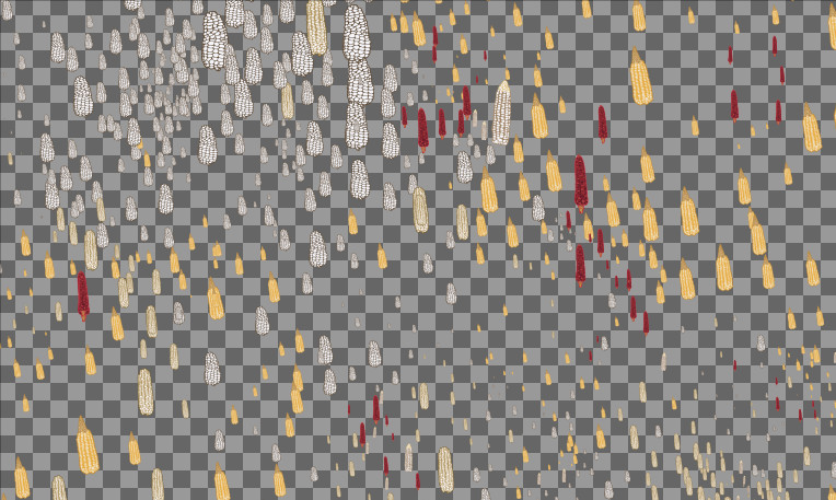
There are 8 different SVG symbols that get used thousands of times in this layer. The SVG specification allows repeating symbols to be “cloned”, which means defining them once in the SVG file and then referring to the original every time the symbol is used. Instead, QGIS draws the symbols every time. So my layer is ripe for optimization. The SVGO command I used goes like this:

svgo cultivos_maiz_municipios.svg --config svgo.config.js -o cultivos_maiz_municipios_opt.svg

In this case, I used a configuration file that specifically asked to reusePaths, which by default is off. My svgo.config.js file was this:

module.exports = {
  plugins: [
    {
      name: "preset-default",
      params: {
        cleanupAttrs: false,
      },
      name: "reusePaths",
    },
  ],
};

After optimizing with SVGO my file went from 104 MB to 9.5 MB, a whopping 91% reduction in size! You may not get such a dramatic reduction in file size and you may not need to optimize your SVGs at all, but you may want to consider adding SVGO to the mix as part of your workflow.

Problem : your vector is still too complex for QGIS

I had an even more complex layer, the one with corn per communal plot. This is the one with the 22,000 symbols, each one being of 8 possible SVG markers (representing one of 8 races of corn) between 24 to 67 KB in size. QGIS was unable to export this vector file: it just silently crashes (not going anywhere near running out of memory), just like when trying to export the whole map. This single layer is hitting some limit in QGIS, but I haven’t even searched for a bug report about it, by this time I already knew what I was trying to do was outside the bounds of the work of the large majority of QGIS users so I just went straight for the workaround (I promise to report or add a comment to that bug soon). So, how to export extra complex vectors from QGIS?

Solution: use clipping in QGIS to make partial exports

The solution is to make partial exports of your composer canvas, small enough so that QGIS can hopefully handle them. There is a somewhat hidden option in the QGIS print composer to “clip” exports of your composer canvas. You first need to make several rectangles on your composer covering your entire canvas. Make sure to use snapping or check the position and size of each rectangle to ensure they cover absolutely the entire surface of your map.

Select your map and then go to the Item Properties tab. The Clipping Settings icon is tucked away at the top:

On the Clipping settings dialog, make sure the Clip to item checkbox is on and choose the name of one of your rectangles.

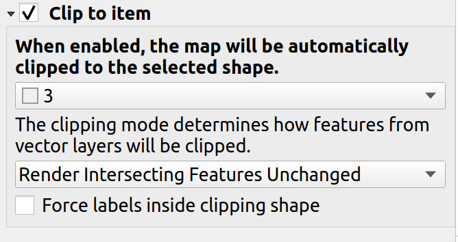
When you export your map a full size SVG is exported but only the content under the selected shape is actually included.

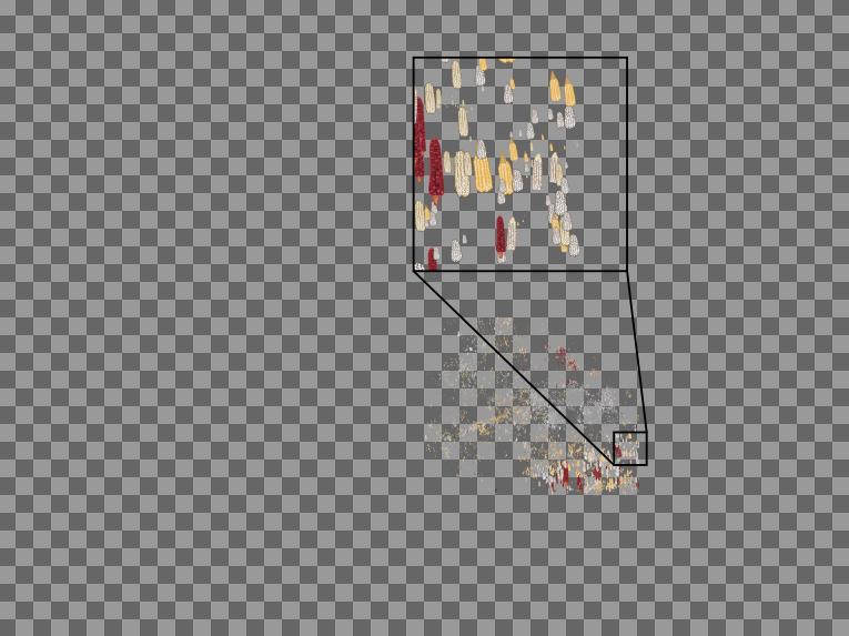
I made a little zoom in so you can see more than a blur (remember this map is to be printed 4 meters wide). Repeat the above steps once for each of your clip shapes. I ended up with 5 files with a total size of 821 MB (about the expected size given the amount of symbols and the size of the SVG markers). After sending them through SVGO (separately) I got a total size of 72 MB, again a reduction in size of 91%.

Could this clipping solution have worked as a way to export the whole map albeit surely with many more than 5 pieces? Who knows, I just thought about it. Let me know if this works for you.

We then rasterize these five vectors (cultivos_maiz_1.svg, cultivos_maiz_2.svg and so on) using the commands explained above: two calls to inkscape to convert one half of each image to bitmaps, then one call to convert to append the images. We can start simplyfying things a bit here, by using && to send a bunch of separate commands in one go without having to sit and wait for each to complete. They will be executed in sequence:

inkscape --export-area=0:0:8390:12548 --export-dpi=300 --export-filename=out_left.png cultivos_maiz_1.svg &&
inkscape --export-area=8391:0:16781:12548 --export-dpi=300 --export-filename=out_right.png cultivos_maiz_1.svg &&
convert -monitor +append out_left.png out_right.png cultivos_maiz_1.png

We end up with 5 bitmaps, all full size, each with a section of the full layer.

Layering images with ImageMagick

So now I have a whole bunch of map layers in PNG format. I need to put them back together with varying levels and modes of transparency, all sorts of masks and things. I know already that I can’t do this in GIMP or Krita, just opening one of these 52438 x 39213 layers takes up a whole lot of time and memory, never mind 15 layers. And I have better things to do.

In the ImageMagick world layering images is called composition. Technically, it involves putting exactly two images together, while setting position, transparencyPlease note that the terms “transparency”, “opacity” and “alpha” may or may not be interchangeable, they may mean different things in ImageMagick and other applications and that could generally drive you nuts., size, and so on. We are working with lossless images (PNG), almost all of them at native resolution, which will not change (with the exception of the shaded relief layer, which is of much lower resolution since it’s derived from SRTM data). This means that I should not have any quality issues as I compose my layers one by one, I just need to plan the process.

The ImageMagick documentation is not the easiest to understand, the syntax is a bit complex and there are not a whole lot of examples online for what I needed to do. So I will just list here some of the commands I used with an explanation of what each section does. Hopefully some of these are what you need for your specific use case.

General points

• All of this is about sequentially adding exactly two layers together. So I made five groups of layers which I then put together in the final step. In this way if I had to change something I only did it for that group of layers and then repeated the final step.
• I chose to use the convert command with the -composite option as opposed to the composite command. They work in different ways, most importantly, layers are listed bottom to top when using convert, and the opposite with composite. Version 7.x of ImageMagick (this tutorial uses 6.x) changes the way of calling commands, so it gets more complicated. Ok, so here we use convert.
• We add -composite to tell ImageMagick to layer the two preceding images (bottom to top) and either output to a file or continue layering with the following image.
• Do not confuse -composite with -compose. We use -compose specifically to indicate options related to transparency.
• I start the list of options with -monitor so that we get a progress % while the command is running. Since I was working with large images and each command takes some time, it is always good to know if things are moving.
• Sometimes I used parentheses to group things, but in the command line they must be preceded by a backslash, so \( this is how it looks \).
• Backslashes \ are also used to make a line break to improve readability, but you can just remove them and write the command in one long line.
• There are surely shorter ways of doing this, but I preferred not to mix too many steps in one command, things got complicated really fast.
• And finally, I don’t understand why some of the things I did worked. Some of it was copied from things I found around in Stack Overflow and other places and they ended up working or were the result of crazy trial and error. It gets really baroque with ImageMagick. So here we go.

Preparing background layers and playing with transparency

The first step was to put together the bottom layers: land use, sentinel satellite images, shaded relief, shore and sea. I started with just land use and shaded relief:

convert -monitor \( land_use.png -channel a -evaluate set 25% \) \
  \( \( -size 52438x39213 xc:white \( -resize 52438x39213 shades_140.png \) -composite \) -channel a -evaluate set 75% +channel \) \
  -compose multiply \
  -composite \
  \( land_use.png -channel a -separate +channel \) -alpha off \
  -compose copy_opacity \
  -composite 1.png

Which means:

1. convert: The ImageMagick command
2. -monitor: Give me a precentage of progress as you do things
3. land_use.png: my bottom layer, an INEGI Mexican land use layer which I have colored so that it blends into the Sentinel image used for neighboring countries: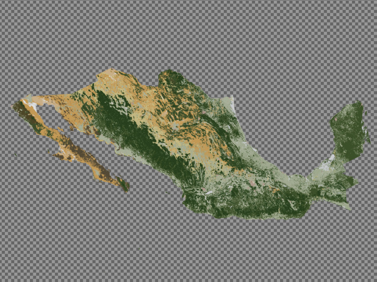
4. -channel a -evaluate set 25%: Give that layer 25% transparency
5. ( ( -size 52438x39213 xc:white ( -resize 52438x39213 shaded_relief.png ) -composite ): take the shaded relief layer, resized to the size of my map and layer it on a white background (white background goes first, order is bottom to top). So there is two layers: a white background and the shaded relief, both the same size, added together with the -composite at the end
6. -channel a -evaluate set 75% +channel ): take the result of the previous step and give it an transparency of 75%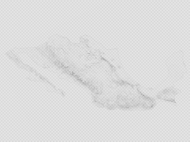
7. -compose multiply -composite: Layer those two images (land_use.png and the one you just made with the white background and the shaded relief at 75%) using the multiply blend mode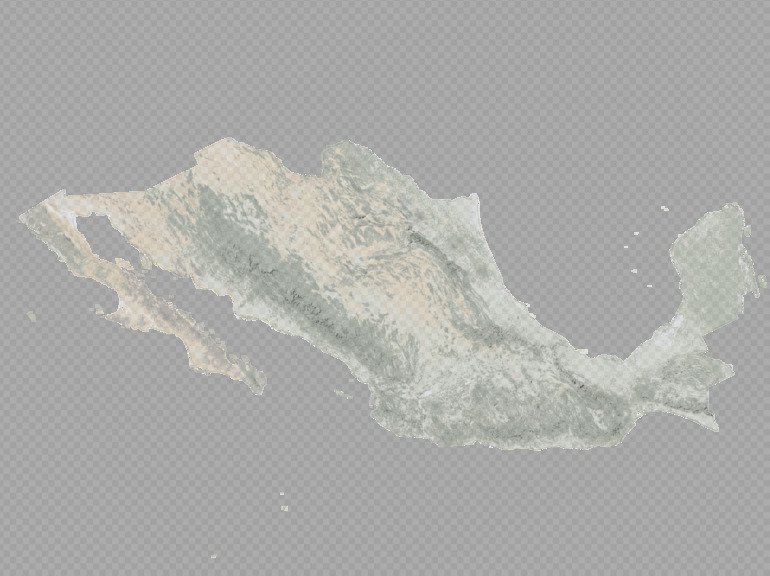
8. \( land_use.png -channel a -separate +channel \) -alpha off -compose copy_opacity -composite 1.png: Take the transparent part (the alpha channel) of land_use.png and copy it to the previous image (land use and shaded relief) and flatten it, thus getting a final image (1.png) with the same transparent parts as the land use layer. This is needed because the shaded relief does not have a transparent sea and we need the sea to be fully transparent for the next step.

Memory usage of this operation peaks at about 51 GB RAM, as ImageMagick does a bunch of processing in memory.

Adding Sentinel and sea images

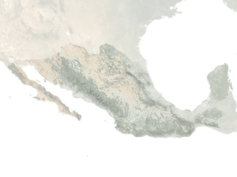
We now take our Sentinel satellite image, which we use for natural color of the US and Guatemala, and has been color corrected using GIMP to match the land use layer used as Mexico background,

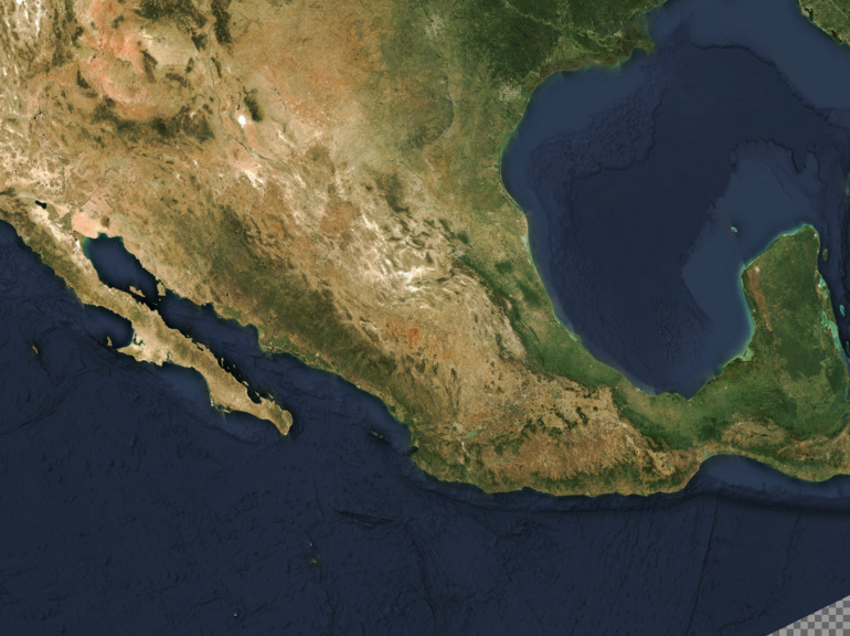
(image credit: European Space Agency - ESA) and layer it with 20% transparency on a white background,

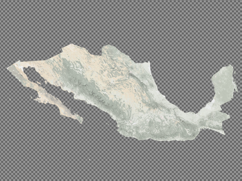
then layer the result of our land use composition above,

We then use a coast mask layer created with QGIS,

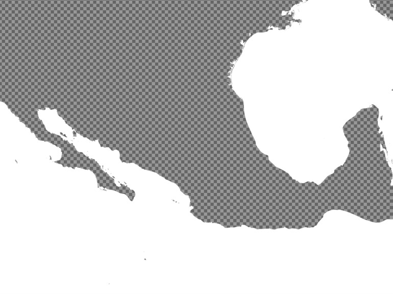
and compose it on top of our Sentinel/land use/shaded relief composition to get rid of the Sentinel sea image,

We finally get our sea layer,

and set it on top of everything:

This is the full command for that step:

convert -monitor -size 52438x39213 xc:white \( sentinel.png -channel a -evaluate set 20% \) -composite 1.png -composite costa_mask.png -composite mar_color_300.png -composite 2.png

I’ll let you deconstruct it into its parts. Each -composite says either:

• layer the previous two things on top of each other (second on top of first) or
• layer the result of the previous step on top of the following thing or
• save the result of the previous step in the following file

The final operation to complete our background is quite simple: just add the coastline, state borders and rivers on top, in that order:

convert -monitor 2.png coastline.png -composite states.png -composite rivers.png -composite 01_BACKGROUND.png

We end this section with a filename for the first of our main components, 01_BACKGROUND.png.

This is the end of Part I of this tutorial. Part II will deal with automating everything using scripting, locating images that are smaller than your canvas and producing the final output. I'd love to hear what you have to say about all this!

Comments

Comments are moderated before they are published.

NEXT >

You can also comment on Twitter.